Google Sheets Conditional Formatting Custom Formula Contains Text

Custom Formula With Text Contains Dokumentredigerare Hjalp

Fwmesgtuxtjflm
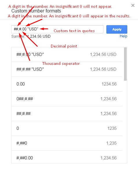
How To Add Custom Text To Number That Can Be Considered In

Google Sheets Shopping List Math Lesson Distance Learning

Google Sheets Bowling Scores Chart Review Distance Learning

Five Steps To Apply Conditional Formatting Across An Entire Row

Formatting based on another range of cells values is a bit more involved.
Google sheets conditional formatting custom formula contains text. In the conditional formatting rules pane select single color. Under format cells if choose the. Note some of the information above may be out of date as google continually add new features to the apps and make cosmetic changes. Use wildcard characters with conditional formatting in google spreadsheets if we want to format text values then the standard text contains condition is essential.
On your computer open a spreadsheet in google sheets. Select the range that you want formatted. You can use special wildcard characters to add some flexibility to the search condition. Select the cells you want to apply format rules to.
Under the format rules select. In the formula field enter the formula. Click on the format menu. Click format conditional formatting.
Click on conditional formatting. B2 35 specify the format by clicking on the formatting style drop down. For an extra use of conditional formatting and custom formulas see my post on using the functions isemail isnumber isurl and not to check that emails addresses etc are ok. Highlight all the cells inside the table and then click on format conditional formatting from the toolbar.
Following are step by step instructions to format a range of cells using values in another range of cells. Navigate the dropdown menu to near the bottom and click conditional formatting. Google sheets conditional formatting based on another cell. From the format cells if drop down select custom formula is.
Using google sheets for conditional formatting based on a range s own values is simple. From the panel that opens on the right click the drop down menu under format cells if and choose custom formula is. A toolbar will open to the right. Go to the format tab.

Excel Tutorial 2019 How To Remove Duplicates Tutorial Excel

Excel Basics 16 Chart Basics Excel Charts Excel Excel

Excel Tutorial 2019 How To Change Cell Background Colour

Formatting A Negative Number With Parentheses In Microsoft Excel

3 Crazy Excel Formulas That Do Amazing Things Docs Templates

Yearly Budget Excel Sheet Instant Download Budget Mac Budgeting

Index Match In Excel Better Alternative To Vlookup Excel

How To Create A Work Schedule In Excel With Images Excel

Excel Basics 16 Chart Basics Excel Charts Excel Excel

Free Excel Spreadsheet For Small Business Accounting And Excel
How To Make A Banner In Microsoft Word How To Make Banners

Mail Merge Address Labels Using Excel And Word Print Address

Best Tv Streaming Apps Disney Vs Apple Tv Vs Netflix Vs Hulu

Handy Accounts Receivable Aging Report Using Excel Accounting
