Google Sheets Conditional Formatting Due Date
Formatting Cells Based On Date Ranges In Google Sheets The Journal
Date Related Conditional Formatting Rules In Google Sheets
Extending Conditional Formatting In Google Sheets Using Dynamic
How To Highlight Cells Based On Expiry Date In Google Sheets

Newco Shift Three Ways To Format Cells In Google Sheets So
Excel Conditional Formatting With Dates 5 Examples Youtube
This is another most commonly occurring date related conditional formatting rules in google sheets.
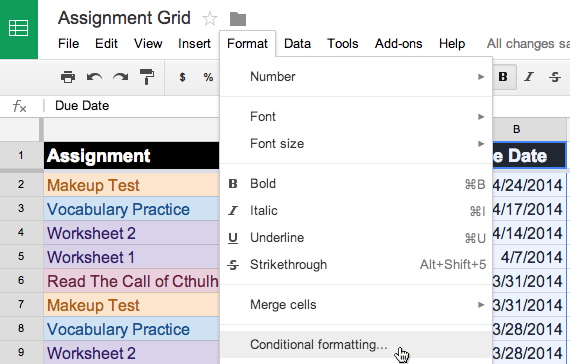
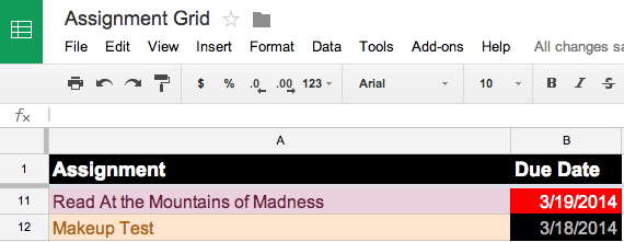
Google sheets conditional formatting due date. I am applying this formatting in a small range a2. Default conditional formatting options in google sheets that doesn t give a lot of options for providing visual cues about date based information such as how far in the future a particular assignment might be due. The above conditional formatting is based on one month cut off date. For example you might say if cell b2 is empty then change that cell s background color to black.
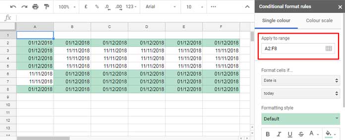
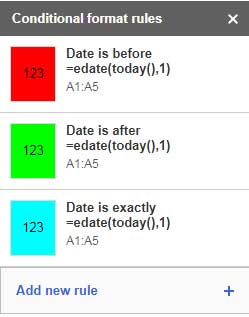
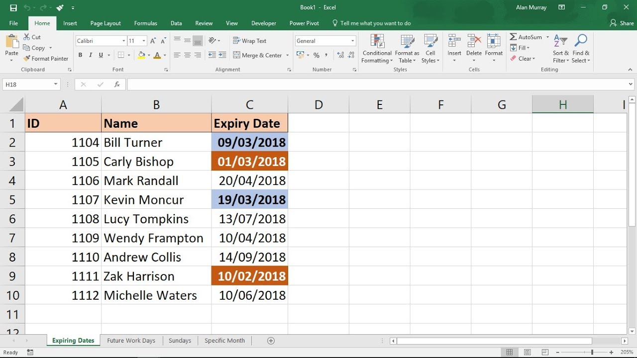
Select the range of cells to which you wish to apply your conditional formatting. Format conditional formatting date is before in the past week red date is after in the past week green date is in the past week orange. Conditional formatting is used to highlight to the reader of the spreadsheet certain values that meet certain criteria. Use conditional formatting with three rules.
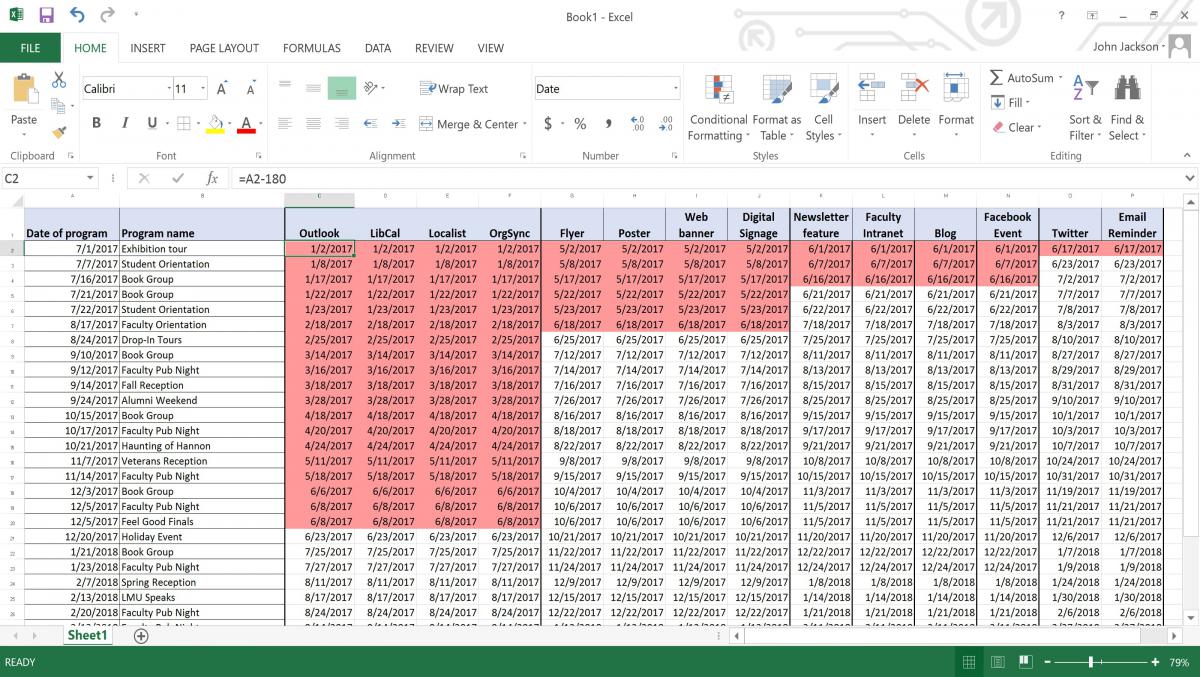
Open the conditional formatting dialog. Suppose you want to highlight column a if the date is between 01 11 2018 and 31 01 2018. Formatting cells based on date ranges in google sheets step 1. Looking to take a column of dates these dates are project end dates compare them to today s date and format them to change color whether they are 60 days prior to end date 30 days prior to equal to end date day of and past end date.
Then you can use the below custom formula in conditional formatting. Now if you want to set 6 months cut off date just change the custom formula as below. Google sheets conditional formatting allows you to change the aspect of a cell that is a cell s background color or the style of the cell s text based on rules you set. New to conditional formatting.
Every rule you set is an if then statement.

Conditional Formatting Due Date Docs Editors Help
Google Sheets Conditional Formatting Based On Another Cell Youtube

Conditional Formatting Of Due Dates Dokumentredigerare Hjalp

Conditional Formatting Based On Dates Is Not Working Correctly

Conditional Formatting Improvements In Google Sheets Youtube
Using Conditional Formatting To Colour Cells In One Column By
Keeping Tabs On Deadlines With Excel S Conditional Formatting

Google Sheets Tips Conditional Date Formatting Youtube

How To Use Conditional Formatting For Colors In Google Sheets
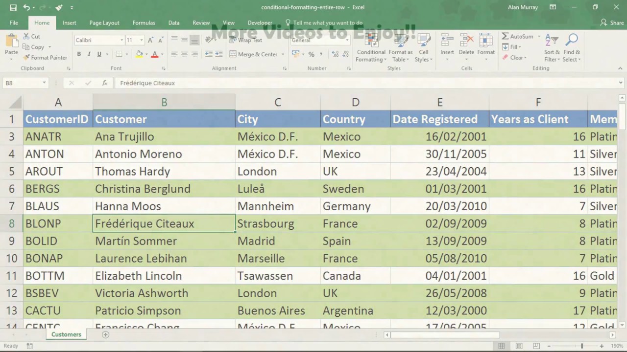
Apply Conditional Formatting To An Entire Row Excel Tutorial

Fill Series Overides Conditional Formatting Docs Editors Help
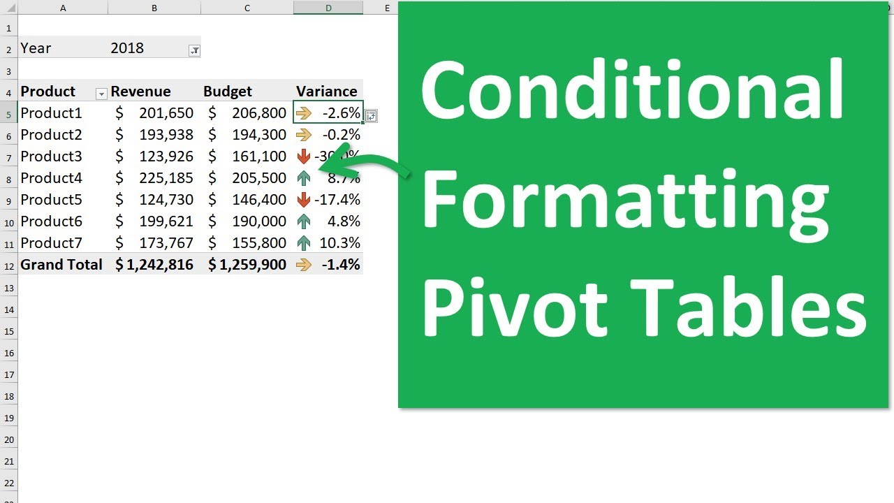
How To Apply Conditional Formatting To Pivot Tables Youtube

Use Conditional Format To Highlight Overdue Dates Youtube

Excel Conditional Formatting Multiple Columns 3 Examples Youtube
